
In many ways, static timing analysis (STA) is more of an art than a science. Methodologists are faced with addressing complex phenomena that impact circuit delay — e.g., signal crosstalk, dynamic I*R supply voltage drop, temperature inversion, device aging effects, and especially (correlated and uncorrelated) process variation between logic cells in a performance-critical path. The uncertainty in clock and data signal arrivals at a storage element at both fast and slow PVT corners necessitated judicious allocation of timing margins, for verification of both setup and hold constraints.
With the progression of process technology, the impact of (global and local) process variation has increased, and thus required a more sophisticated solution, in lieu of a simple margining approach. The STA methodologists needed to address how to reflect statistical variation in the arrival time propagation calculations, and the determination of a “confidence level” for arrival-to-setup/hold checks. (Lesser timing margin values would still be applicable to other phenomena besides process variation.)
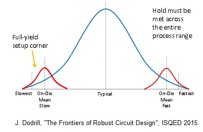
As illustrated in the figure below, the definition of a PVT corner for timing analysis was expanded to include a local, intra-die delay variation component. An on-die PVT “global mean” is defined, with a local distribution around that reference. Note that this global mean is somewhat artificial, as it represents a value around which measured local variation is added to align with the total measured process variation data.

Designing to a global “n-sigma” target at the far extremes of the process distribution would be too pessimistic, and increasingly difficult for designers to close timing. An overall global mean + local n-sigma method is used instead. (Note in the figure that the author is recommending that a very high-sigma still be applied for hold time checks at the fast PVT corner, due to the unforgiving behavior of a hold time failure.)
Recently, I had the distinct pleasure of chatting with Igor Keller, Distinguished Engineer in the Silicon Signoff and Verification Group at Cadence. He and his colleagues presented a paper at this year’s Tau Workshop, which caught my eye, entitled “Importance of Modeling Non-Gaussianities in Static Timing Analysis in sub-16nm Technologies”. The Tau Workshop is the premier venue for STA methodologists and EDA tool developers, to discuss how current challenges in the field are being addressed — it is definitely worth attending/tracking (link).
Igor reviewed some of the recent history of STA development, then highlighted a critical area that his team has been addressing.
First, a brief recap…
Full “statistical” STA (SSTA) was proposed over a decade ago, yet the implementation proved to be extremely complex. The delay and output slew characterization of cells as a function of loading and input signal slew — the backbone of STA — was costly. The propagation of full statistical arrival probability distributions was intricate. It required mathematical interpretation of the probability distribution of arrivals and slews at cell pins and the addition of probability distributions for cell delays, as timing analysis progressed through the network timing graph. In addition to timing signoff, physical implementation tools also need to integrate the timing engine as part of their iterative design optimizations. The adverse performance impact of full SSTA made utilization during physical design cumbersome.
An alternative method emerged as more practical, and still sufficient — Advanced On-Chip Variation (AOCV) analysis. AOCV utilizes the concept of stage depth in STA calculations, using the levelization of gates in a logic path to determine the depth number. A derate delay multiplier based upon logic path depth is applied to the local delay distribution to reflect the correlated variation of on-die circuits — the greater the number of gates in the path, the higher the assumed correlation. The derate multiplier decreases with the stage delay number. (Some AOCV approaches also include location-based derate tables, to further reflect local correlation factors when the physical extent of the path is bounded.) This methodology has gained acceptance, with STA tool functionality and with the foundries providing support for representing process variation in the form of a global mean and local derate tables.
An enhancement to existing OCV methods has been promoted by the Liberty Technical Advisory Board (TAB), a consortium of company representatives working on standards for circuit modeling (link).
The Liberty Variation Format (LVF) introduces a local standard deviation sigma into the cell characterization library data, and a table format for sigma as a function of input pin slew and output load is provided. This characterization approach allows the STA methodologist a general method to close setup/hold timing yield independently to “n-sigma”, generating corresponding derates.
(Note that there is certainly process variation impacting the setup and hold constraints at the clock/data inputs of a storage element. This variation is typically incorporated with the other timing margin factors.)
Igor highlighted that the AOCV and LVF n-sigma approach used to date has assumed Gaussian, or normal, variation distribution, as depicted above. In advanced process nodes, the variations are distinctly non-Gaussian. Additionally, the trend to operate logic circuits at reduced VDD supply voltage for low-power applications also results in non-Gaussian delay distributions. This necessitates a new approach, to the representation of the statistical “tail” of the arrival time distribution at a test point in the timing graph.
The Cadence team’s presentation at Tau highlighted how non-Gaussian cell distributions can be accurately and efficiently represented, and how the subsequent calculations of (non-Gaussian) delay, slew, and arrival time variations are propagated through the network graph.
The foundation for their approach begins with the same generation technique used for library cell characterization of delays and slews. Monte Carlo Spice simulations of cells (using advanced parameter sampling techniques) provide the discrete data. From this dataset, the following statistical parameters are calculated:
- overall mean (based upon the global process mean above)
- “shifted” mean (of the non-Gaussian data)
- variance (aka, the statistical 2nd moment; the square of the standard deviation)
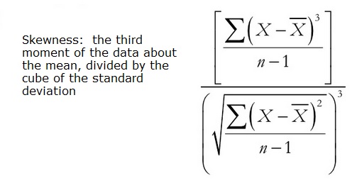
- skewness (the statistical 3rd moment)
The calculation is extendible — the 4th moment, or kurtosis, could also be derived for the data distribution. Further, to accelerate the adoption of this approach, these values can be represented in a similar table format to the current LVF data.
Timing graph analysis now proceeds with delay/slew calculation and the propagation of arrival times. (Although our discussion focused on forward propagation of arrival times, Igor indicated the same technique applies to backward propagation slack calculation, as well.)
The main STA network timing methods are graph-based analysis (GBA) and path-based analysis (PBA, which should always be “bounded” by a GBA calculation). These methods require algorithms for min/max/sum calculations for cell pin arrival and pin-to-pin delay arcs. The Tau paper goes into detail on these calculations, using the best representation for the non-Gaussian distribution of the shifted mean, variance, and skewness values — e.g., a log-normal or a Cauchy distribution. The key is that these calculations do not adversely impact runtime performance.
The tail of the arrival data distribution at a test point provides a statistical probability of the timing yield, represented as a “quantile” for non-normal distributions. (Three sigma for a normal distribution corresponds to the 0.99865 quantile.)
Igor provided examples of the distinctly non-Gaussian cell delay values, including circuits operating at low VDD at advanced nodes. The figures below highlight the fact that the “0.99865 quantile delay” is far from the (Gaussian mean + 3 sigma) calculation, especially at low VDD.
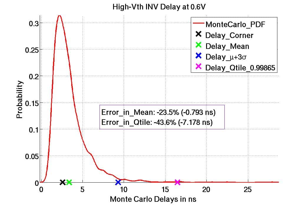
Example of the delay distribution for a high Vt inverter cell @ VDD=0.6V. Note the difference between the (Gaussian) 3-sigma delay and the non-Gaussian 0.99865 quantile delay, which reflects the same timing yield.
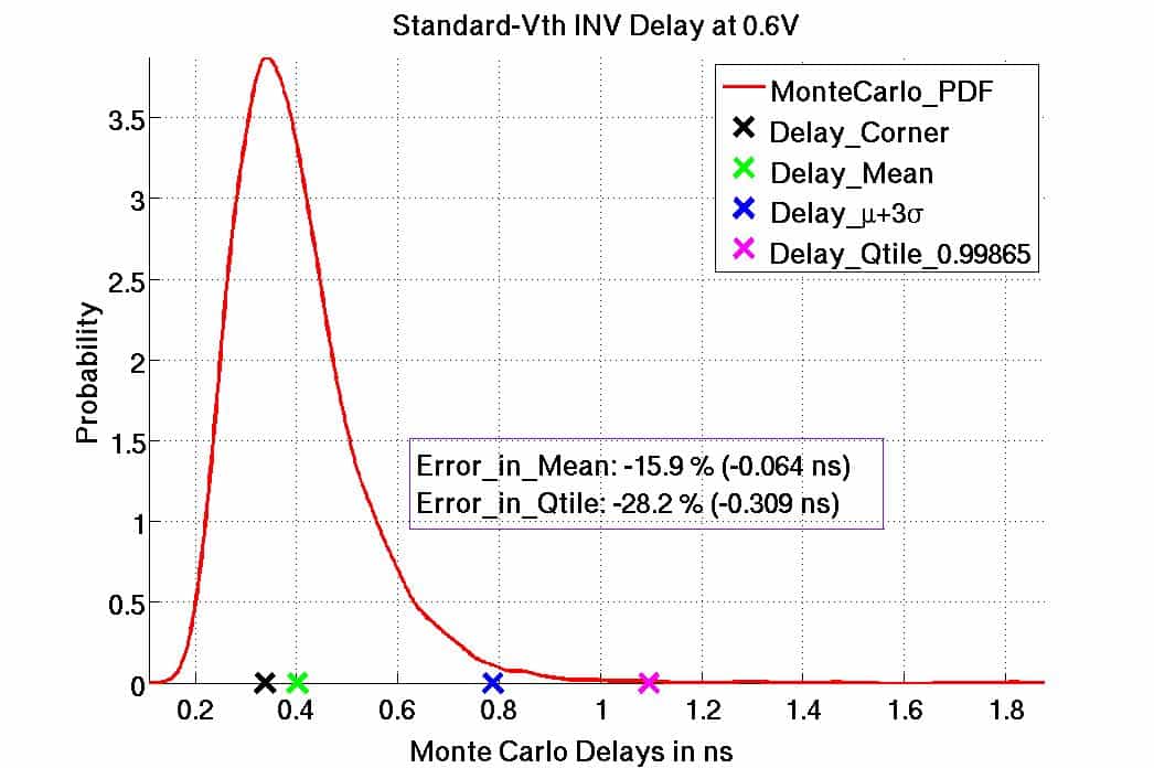
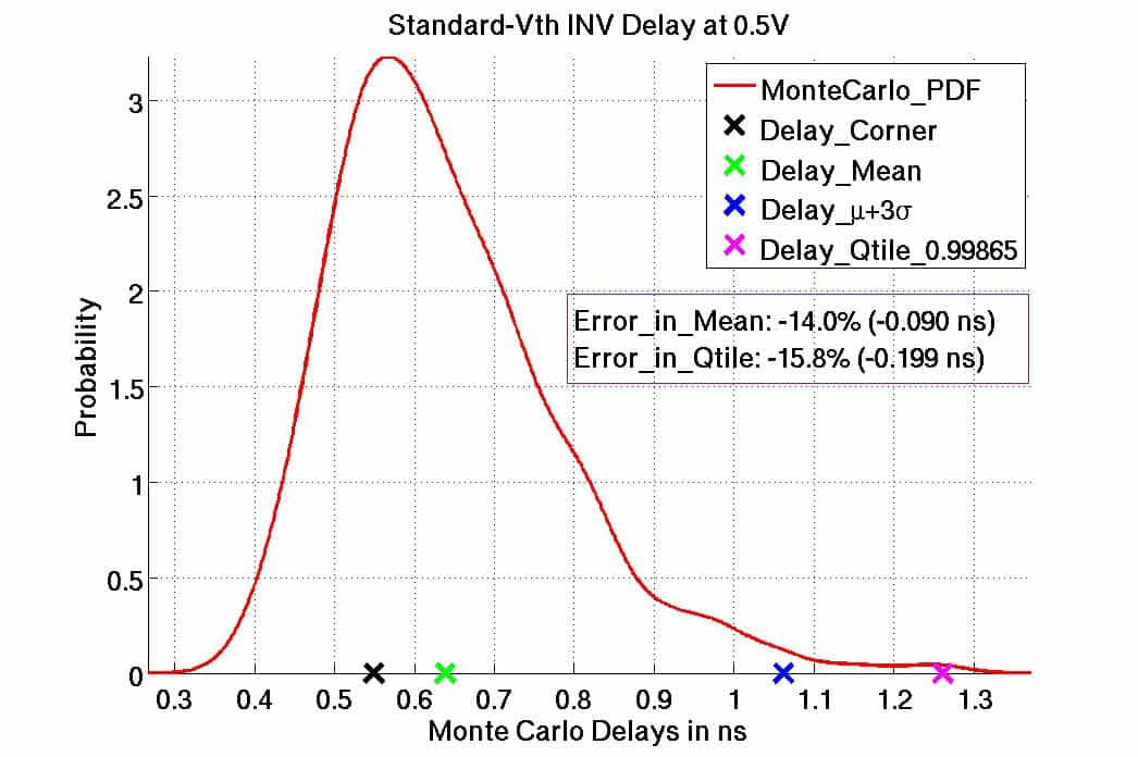
Delay distributions for standard Vt inverter cells. The second example uses 7nm device models, operating at an extremely low VDD. Again, note the difference between Gaussian and 0.99865 quantile delays.
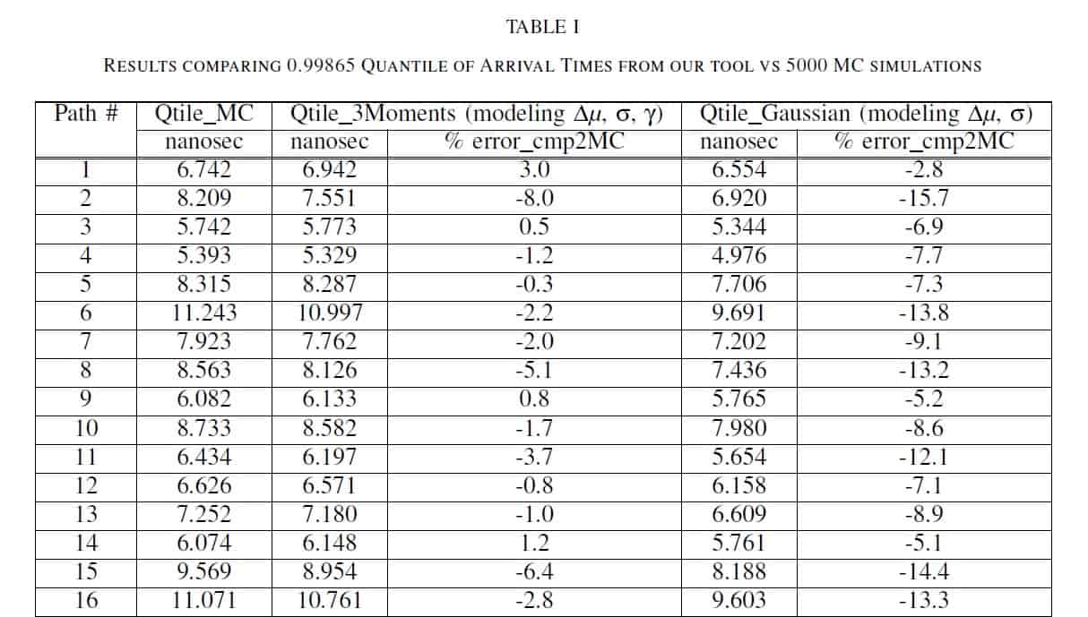
The Tau paper provided comparisons between reference Monte Carlo Spice simulations of full paths, to the prediction from the Gaussian and non-Gaussian distribution cell library LVF models — a few examples are excised from that paper in the figure below. The benefits of the improved non-Gaussian delay model are clear.
Cadence has integrated the non-Gaussian LVF extension support into their Tempus STA signal tool, and as the integrated timing engine in their Innovus implementation platform. They are working with the Liberty consortium to extend the current LVF definition as a standard.
STA is evolving to provide methodologies that support accurate timing yield signoff, in the face of increasing variation, while maintaining efficiency of library generation and delay calculation/propagation. That said, there are plenty of challenges ahead. Igor provided additional insights,
“We are working on several facets of STA — improved modeling of crosstalk, better support for multiple-input switching effects, better inclusion of aging models.”
Look for compelling advances in timing yield analysis in the future. For more information on Cadence Tempus, please follow this link.
-chipguy
Share this post via:


Comments
0 Replies to “The Latest in Static Timing Analysis with Variation Modeling”
You must register or log in to view/post comments.